Google Sheets attendance tracker template

The finished tracker from the video, ready to use. Pick P, A or L for each day. The colours, counts, attendance rate and chart update by themselves. It has room for 30 students and four school weeks.

Download the template (.xlsx)

Open it in Google Sheets

1. In Google Drive, click New → File upload and pick the file.
2. Double-click it to open it.
3. Click File → Save as Google Sheets.
4. Type your students' names over the sample names in the Attendance tab.

What's inside

• Attendance — one row per student, one column per day. Every day cell is a P / A / L dropdown. Present is green, absent is red, late is amber.
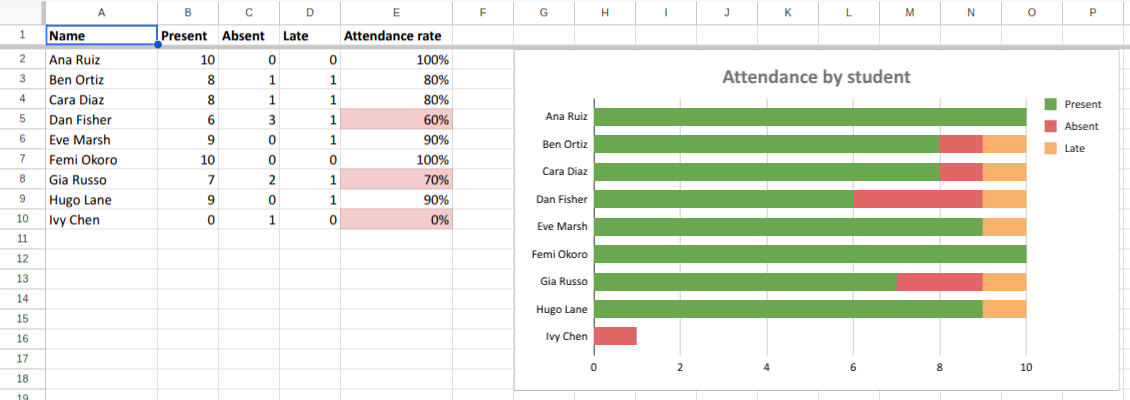
• Summary — each student's present, absent and late counts and their attendance rate. A rate under 80% turns red. The chart shows everyone at once.
• Codes — the list the dropdowns read from.

The formulas

These are the formulas typed in the video, for row 2 of the Summary tab:

=COUNTIF(Attendance!B2:K2,"P")

=COUNTIF(Attendance!B2:K2,"A")

=COUNTIF(Attendance!B2:K2,"L")

=B2/SUM(B2:D2)

The rate is present days out of every day marked, so a late day lowers it. Format the column as a percent.

The template uses the same formulas with two changes. It has empty rows, and the video didn't. So each formula is wrapped to stay blank on a row with no name, like =IF($A2="", "", COUNTIF(Attendance!$B2:$U2, "P")). The red flag is the custom formula =AND(ISNUMBER($E2), $E2<0.8), not "Less than 0.8", so it only colours real rates.

Changing it

• A different cut-off. Select the Summary rates, open Format → Conditional formatting, and change the 0.8.
• More than 30 students. Copy the last Summary row down. Then widen the ranges in Data → Data validation and Format → Conditional formatting on the Attendance tab, and the chart's data range.
• Another code, like E for excused. Add it to the Codes tab. Widen the dropdown's range in Data → Data validation. Then add a Summary column with another COUNTIF.

The counting half is explained on the COUNTIF reference page.